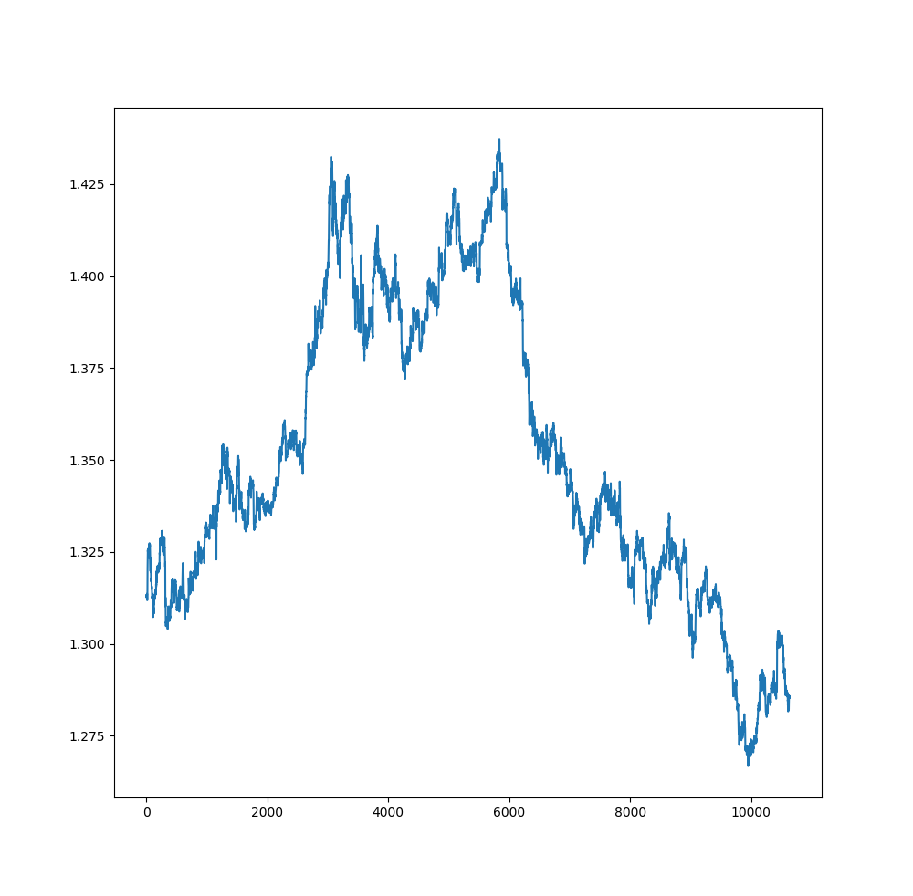
RandomForest is a supervised machine learning algorithm that uses the ensemble machine learning in making predictions. In this post I will try to build a RandomForest Algorithmic Trading Model can see if we can achieve above 80% accuracy with it. The idea is to build an algorithmic trading strategy using Random Forest algorithm. Then we backtest that strategy and check the equity curve. This is an educational post. The purpose is to teach you how to develop and then backtest an algorithmic trading strategy. In this algorithmic trading strategy we will be using RandomForests algorithm. So let’s discuss it first. Below you can find the GBPUSD 30 Minute 10K bar data comprising almost one year. Are you interested in cryptocurrencies? Read this post on how Ethereum gained 8000% last year.
This is a trend trading strategy. Trend is your friend until it bends. This is what the professional traders say to new traders. Trend trading is where professional traders make their fortunes. However predicting trends is a challenging task. Long term trend prediction in modern markets is a difficult and challenging task as there are many uncertainties. These uncertainties are mostly political events happening around the world that can impact that particular financial market. Breaking news that can impact a certain financial market will have sudden impact and cannot be predicted ahead of time. Financial markets are dynamic non linear system that are being driven by many factors that are difficult to figure out and measure in most cases. So we take financial markets as random and chaotic dynamic systems.
In recent years several people have tried to predict the financial markets using machine learning techniques. We will consider the paper: Predicting the direction of the stock market prices using random forests by Luckyson Khaidem, Sudeepa Roy Dey and others. The authors claim achieving a predictive accuracy of 90% which is astounding. So let’s discuss the paper in this post. Then we develop the Python code that implements the Random Forest Trend Prediction Algorithm and check for ourselves how good is the predictive accuracy of the algorithm in reality. Most of the time you will find good research papers on quantitative finance that you can use to develop your algorithmic trading strategies based on them. Developing the algorithmic trading strategies will of course test your mathematical and programming skills. But the rewards can be very good if you hit upon a good algorithmic trading strategy idea that makes good profits for you. The quoted paper uses the following indicators:
- Relative Strength Index RSI is a popular momentum oscillator.
- Stochastic Oscillator SO another popular momentum oscillator.
- William %R
- Moving Average Convergence Divergence
- Price Rate of Change
- On Balance Volume
We will be using these indicators to predict the Target variable which will be the trend for the next 1,5,10,14 and 30 bars. Before we continue let’s become familiar with the Random Forest Algorithm
Random Forest Algorithm
What is a Random Forest? You might be thinking we will be hunting in a dark forest. Sort off. Not physically but in a statistical sense. Random Forest Algorithm is an Ensemble Learning Algorithm that first builds Decision Trees. Decision Trees has long been a popular algorithm. Decision Trees first got introduced in 1970s and have been popular since then. Decision Tree is an intuitive algorithm and translates the prediction into rules which can be easily understood by laymen. You don’t need to do complex mathematical transformation before using Decision Trees algorithm which is one reason why it has been popular. Decision Trees algorithm splits the features using a number of statistical measurements. Each split is determined in such a way that improves the sample. The statistical measures usually used to make splitting decisions is the gini impurity, information gain and the variance reduction. Information gain is based on the information entropy function. Long story short, decision trees split data in such a manner that is minimizes the entropy.
Decision Trees have on problem. They are prone to overfitting. We traders try to build trading rules in our trading strategies. For example, buy when RSI is oversold and below 20 and sell when RSI is overbought and above 80. Sounds simple. We can add more rules like buy when RSI is between 20 and 30 and MACD is changing color. Similarly sell when RSI is between 80 and 70 and MACD is changing color. Now most of the time you will find that these rule based trading strategy gives a losing trade. Why? We are overfitting. These rules are like decision trees which also overfit most the time. Overfitting is a curse of machine learning. When you overfit the data, the predictions are poor on unseen data as the algorithm failed to separate the signal from random noise. Read this post on how to do algorithmic trading with Oanda Python API.
Decision Trees have more variance than bias. In the presence of noisy data, you can improve decision trees to retrain the algorithm using only correctly predicted cases and build a separate tree for the misclassified cases. Another method to improve the predictive accuracy of a decision tree is to build number of trees from the same sampled data and then averaging the results. In case of classification, the majority predicted class is taken as the output class. In Random Forest we are using bootstrap sampling to build multiple trees that are uncorrelated to each other. So this is what we do in Random Forest algorithm. We bootstrap the training data multiple times and build a decision tree each time. We also compute the performance of the trees by using training data that we didn’t use in building the tree. This is known as Out of Bag Estimated (OOB). Once we have build the trees, we use voting to predict the outcome. Using the above method we are able to reduce the variance and the bias problem that we have in decision trees. This was some theory. However, you should become more familiar with the Random Forest Classifier if you really want to build an algorithmic trading strategy based on it.
Let’s start. First we need to read the data. You should have Python installed on your computer. Use Anaconda to install Python. I am using Visual Studio Code as the IDE. You can use Spyder. First we import the numpy and pandas libraries. Numpy and Pandas are very powerful libraries. You should become familiar with them as much as possible as all the work is done by these two libraries. Then we using pandas to read the GBPUSD 30 Minute csv file that I have download from MT4 History Center and saved on my hard drive. Pandas reads it and you can see below the first few rows of prices in the data and the last few rows of files in the data.
>>> from __future__ import division
>>> import pandas as pd
>>> import numpy as np
>>> import matplotlib.pyplot as plt
>>>
>>> from scipy import signal
>>> #load the data for backtesting
... #define function to read the data from the csv file
...
>>> def get_data(currency_pair, timeframe):
...     link='D:/Shared/MarketData/{}{}.csv'.format(currency_pair,\
...                                 timeframe)
...     data1 = pd.read_csv(link, header=None)
...     data1.columns=['Date', 'Time', 'Open', 'High', 'Low',
...                 'Close', 'Volume']
...     # We need to merge the data and time columns
...     # convert that column into datetime object
...     data1['Datetime'] = pd.to_datetime(data1['Date'] \
...             + ' ' + data1['Time'])
...     #rearrange the columnss with Datetime the first
...     data1=data1[['Datetime', 'Open', 'High',
...                     'Low', 'Close', 'Volume']]
...     #set Datetime column as index
...     data1 = data1.set_index('Datetime')
...     return(data1)
...
>>> df = get_data('GBPUSD', 30)
>>> df.shape[0]
10682
>>> df.shape[1]
5
>>> df.head()
                        Open     High      Low    Close  Volume
Datetime
2017-10-24 15:30:00  1.31195  1.31260  1.31195  1.31215     750
2017-10-24 16:00:00  1.31216  1.31236  1.31144  1.31203     652
2017-10-24 16:30:00  1.31202  1.31361  1.31202  1.31314     685
2017-10-24 17:00:00  1.31313  1.31315  1.31182  1.31284     568
2017-10-24 17:30:00  1.31282  1.31352  1.31221  1.31221     488
>>> df.tail()
                        Open     High      Low    Close  Volume
Datetime
2018-09-05 10:00:00  1.27921  1.28119  1.27886  1.28118    1241
2018-09-05 10:30:00  1.28117  1.28268  1.28058  1.28227    1137
2018-09-05 11:00:00  1.28228  1.28263  1.28138  1.28146     934
2018-09-05 11:30:00  1.28147  1.28282  1.28117  1.28191     931
2018-09-05 12:00:00  1.28198  1.28235  1.28135  1.28148     793
>>>
It is always a good idea to be familiar with how to code your technical indicators. I have done that. You can also use the TA-LIB python library which has all the technical indicators predefined as functions. We will be using the Relative Strength Index, Price Rate of Change, Stochastic Oscillator, Williams %R, On Balance Volume and the Detrend which is just a scikit-learn module that we have used to detrend price and make it stationary. Now that we have read the data we need to define the different technical indicator functions that we do below:
>>> #Trading Strategy Technical Analysis Functions
... #Calculate Relative Strength Index (RSI)
...
>>> def RSI(df, n):
...     '''
...     Relative Strength Index of a given financial time series
...     for a given period length
...     :param dataframe: df
...     :param period: n
...     :return df with rsi:
...     '''
...     rsi=[]
...     diff = np.diff(df.Close)
...     # length is 1 less than the all_prices
...     for i in range(n):
...         rsi.append(None)
...         # because RSI can't be calculated
...         # until period prices have occured
...     for i in range(len(diff) - n + 1):
...         avgGain = diff[i:n + i]
...         avgLoss = diff[i:n + i]
...         avgGain = abs(sum(avgGain[avgGain >= 0]) / n)
...         avgLoss = abs(sum(avgLoss[avgLoss < 0]) / n)
...         if avgLoss == 0:
...             rsi.append(100)
...         elif avgGain == 0:
...             rsi.append(0)
...         else:
...             rs = avgGain / avgLoss
...             rsi.append(100 - (100 / (1 + rs)))
...     df['RSI']=rsi
...     return df
... #Calculate Price Rate of Change (PROC)
...
>>> def PROC(df,n):
...     '''
...     Price Rate of Change of a given financial time series
...     for a given period length
...     :param dataframe: df
...     :param period: n
...     :return proc:
...     '''
...     proc = []
...     price = list(df.Close)
...     for i in range(n):
...         proc.append(None)
...         # because proc can't be calculated
...         # until period prices have occured
...     for i in range(len(price) - n):
...         if len(price) <= n:
...             proc.append(None)
...         else:
...             calculated = (price[i + n] - price[i])/price[i]
...             proc.append(calculated)
...     df['PROC']=proc
...     return df
... #Calculate Stochastic Oscillator
...
>>> def SO(df,n):
...     so = []
...     price = list(df.Close)
...     for i in range(n):
...         so.append(None)
...     for i in range(len(price) - n):
...         C = price[i]
...         H = max(price[i:i+n])
...         L = min(price[i:i+n])
...         so.append(100 * ((C - L) / (H - L)))
...     df['SO']=so
...     return df
... #calculate Williams % R Oscillator
...
>>> def Williams_R(df,n):
...     '''
...     Williams %R
...     Calculates fancy shit for late usage. Nice!
...
...     EXAMPLE USAGE:
...     data = pandas.read_csv("./data/ALL.csv", sep=",",
...     header=0,quotechar='"')
...     wr = Williams_R(data)
...     print(wr)
...
...     '''
...     wr = []
...     price = list(df.Close)
...     for i in range(n):
...         wr.append(None)
...         # because proc can't be calculated
...         # until period prices have occured
...     for i in range(n-1,len(price)-1):
...         C = price[i]
...         H = max(price[i-n+1:i])
...         L = min(price[i-n+1:i])
...         wr_one = (
...             ((H - C)/ (H - L)) * -100
...         )
...         if wr_one <=-100:
...             wr.append(-100)
...         elif wr_one >= 100:
...             wr.append(100)
...         else:
...             wr.append(wr_one)
...     df['WR']=wr
...     return df
... #Calculate the Target label that we will predict
...
>>> def calculate_targets(df, n):
...     targets = []
...     price = list(df.Close)
...     for i in range(0, len(price)-n):
...         targets.append(np.sign(price[i+n] - price[i]))
...     for i in range(len(price)-n, len(price)):
...         targets.append(None)
...     df["Target({})".format(n)] = targets
...     return df
... #Calculate On Balance Volume Indicator
...
>>> def On_Balance_Volume(df):
...     '''
...     On Balance Volume
...     '''
...     obv = []
...     price = list(df.Close)
...     volume = list(df.Volume)
...     obv.append(df.Volume.iloc[0])
...     for i in range(1,len(price)):
...         C_old = price[i-1]
...         C = price[i]
...         if(C > C_old):
...             obv.append(obv[i-1]+ volume[i])
...         elif (C < C_old):
...             obv.append(obv[i - 1] - volume[i])
...         else:
...             obv.append(obv[i-1])
...     df['OBV']=obv
...     return df
...
>>> def detrend(df):
...     trend = None
...     price = list(df.Close)
... #   trend.append(signal.detrend(price))
...     if(trend is None):
...         trend = list(signal.detrend(price))
...     else:
...         trend.extend(signal.detrend(price))
...     print("len(trend):{} len(df['Symbol']):{}".\
...     format(len(trend),len(price)))
...     print("len(trend):{} len(df):{}".\
...     format(len(trend),len(df)))
...     df['detrendedClose'] = trend
...     return df
...
>>>
Now that we have defined the technical indicators that we will be using in developing our trading strategy, we build our feature that we will use to make the predictions. Target is the label that we want to predict. We calculate six targets, 1 step ahead, 3 step ahead, 5 step ahead, 10 step ahead and 14 step ahead and 30 step ahead. We want to know the market direction after 1 step, 3 steps, 5 steps , 10 steps, `4 steps and 30 steps. Now we need to add the technical indicators to the dataframe.
>>> df1 = RSI(df,14)
>>> print("RSI: Done")
RSI: Done
>>> df1 = PROC(df, 14)
>>> print("PROC: Done")
PROC: Done
>>> df1 = SO(df,14)
>>> print("SO: Done")
SO: Done
>>> df1 = Williams_R(df, 14 )
>>> print("Williams_R: Done")
Williams_R: Done
>>> df1 = On_Balance_Volume(df)
>>> print("On Balance Volume: Done")
On Balance Volume: Done
>>> df1["EWMA"] = pd.ewma(df.Close, com=.5)
__main__:1: FutureWarning: pd.ewm_mean is deprecated for Series and will be
removed in a future version, replace with
        Series.ewm(com=0.5,adjust=True,min_periods=0,ignore_na=False).mean()
>>> print("EWMA: Done")
EWMA: Done
>>> df1 = detrend(df)
len(trend):10682 len(df['Symbol']):10682
len(trend):10682 len(df):10682
>>> print("Date detrend: Done")
Date detrend: Done
>>> df1.head()
                        Open     High      Low    Close  Volume  RSI  PROC  \
Datetime
2017-10-24 15:30:00  1.31195  1.31260  1.31195  1.31215     750  NaN   NaN
2017-10-24 16:00:00  1.31216  1.31236  1.31144  1.31203     652  NaN   NaN
2017-10-24 16:30:00  1.31202  1.31361  1.31202  1.31314     685  NaN   NaN
2017-10-24 17:00:00  1.31313  1.31315  1.31182  1.31284     568  NaN   NaN
2017-10-24 17:30:00  1.31282  1.31352  1.31221  1.31221     488  NaN   NaN

                     SO  WR  OBV      EWMA  detrendedClose
Datetime
2017-10-24 15:30:00 NaN NaN  750  1.312150       -0.064344
2017-10-24 16:00:00 NaN NaN   98  1.312060       -0.064460
2017-10-24 16:30:00 NaN NaN  783  1.312808       -0.063345
2017-10-24 17:00:00 NaN NaN  215  1.312829       -0.063640
2017-10-24 17:30:00 NaN NaN -273  1.312415       -0.064265
>>> df1.tail()
                        Open     High      Low    Close  Volume        RSI  \
Datetime
2018-09-05 10:00:00  1.27921  1.28119  1.27886  1.28118    1241  29.202773
2018-09-05 10:30:00  1.28117  1.28268  1.28058  1.28227    1137  35.055644
2018-09-05 11:00:00  1.28228  1.28263  1.28138  1.28146     934  33.536122
2018-09-05 11:30:00  1.28147  1.28282  1.28117  1.28191     931  35.211268
2018-09-05 12:00:00  1.28198  1.28235  1.28135  1.28148     793  34.370478

                         PROC          SO          WR   OBV      EWMA  \
Datetime
2018-09-05 10:00:00 -0.003733   99.260355 -100.000000 -8888  1.280780
2018-09-05 10:30:00 -0.002924  100.000000  -71.745562 -7751  1.281773
2018-09-05 11:00:00 -0.003368   97.604790  -55.089820 -8685  1.281564
2018-09-05 11:30:00 -0.003103   99.251497  -67.215569 -7754  1.281795
2018-09-05 12:00:00 -0.003360   97.754491  -60.479042 -8547  1.281585

                     detrendedClose
Datetime
2018-09-05 10:00:00       -0.043199
2018-09-05 10:30:00       -0.042104
2018-09-05 11:00:00       -0.042909
2018-09-05 11:30:00       -0.042454
2018-09-05 12:00:00       -0.042879
>>> df1 = calculate_targets(df, 1)
>>> df1 = calculate_targets(df, 3)
>>> df1 = calculate_targets(df, 5)
>>> df1 = calculate_targets(df, 10)
>>> df1 = calculate_targets(df, 14)
>>> df1 = calculate_targets(df, 30)
>>> print('Targets Done - except 60')
Targets Done - except 60
>>> df1=df1.dropna()
>>> df1.head(10)
                        Open     High      Low    Close  Volume        RSI  \
Datetime
2017-10-24 23:00:00  1.31301  1.31324  1.31250  1.31308     378  57.276995
2017-10-24 23:30:00  1.31309  1.31328  1.31265  1.31291     360  56.832298
2017-10-25 00:00:00  1.31289  1.31317  1.31259  1.31267     621  45.780969
2017-10-25 00:30:00  1.31262  1.31264  1.31199  1.31261     659  47.842402
2017-10-25 01:00:00  1.31263  1.31302  1.31239  1.31294     547  57.256461
2017-10-25 01:30:00  1.31295  1.31331  1.31284  1.31314     377  60.273973
2017-10-25 02:00:00  1.31315  1.31336  1.31276  1.31334     371  49.376559
2017-10-25 02:30:00  1.31333  1.31363  1.31313  1.31322     362  59.281437
2017-10-25 03:00:00  1.31314  1.31325  1.31284  1.31291     391  55.000000
2017-10-25 03:30:00  1.31284  1.31346  1.31251  1.31345     429  55.000000

                         PROC          SO         WR   OBV      EWMA  \
Datetime
2017-10-24 23:00:00  0.000709    8.823529 -28.676471  -771  1.313069
2017-10-24 23:30:00  0.000671    0.000000 -22.794118 -1131  1.312963
2017-10-25 00:00:00 -0.000358   80.769231 -36.923077 -1752  1.312768
2017-10-25 00:30:00 -0.000175   57.692308 -55.384615 -2411  1.312663
2017-10-25 01:00:00  0.000556    9.230769 -60.000000 -1864  1.312848
2017-10-25 01:30:00  0.000800    0.000000 -34.615385 -1487  1.313043
2017-10-25 02:00:00 -0.000038  100.000000 -29.761905 -1116  1.313241
2017-10-25 02:30:00  0.000472    6.329114   1.282051 -1478  1.313227
2017-10-25 03:00:00  0.000274    0.000000 -15.189873 -1869  1.313016
2017-10-25 03:30:00  0.000274   65.753425 -58.904110 -1440  1.313305

                     detrendedClose  Target(1)  Target(3)  Target(5)  \
Datetime
2017-10-24 23:00:00       -0.063346       -1.0       -1.0        1.0
2017-10-24 23:30:00       -0.063511       -1.0        1.0        1.0
2017-10-25 00:00:00       -0.063746       -1.0        1.0        1.0
2017-10-25 00:30:00       -0.063801        1.0        1.0        1.0
2017-10-25 01:00:00       -0.063467        1.0        1.0        1.0
2017-10-25 01:30:00       -0.063262        1.0       -1.0        1.0
2017-10-25 02:00:00       -0.063057       -1.0        1.0       -1.0
2017-10-25 02:30:00       -0.063172       -1.0       -1.0        1.0
2017-10-25 03:00:00       -0.063477        1.0        1.0        1.0
2017-10-25 03:30:00       -0.062932       -1.0        1.0       -1.0

                     Target(10)  Target(14)  Target(30)
Datetime
2017-10-24 23:00:00         1.0         1.0         1.0
2017-10-24 23:30:00         1.0        -1.0         1.0
2017-10-25 00:00:00         1.0        -1.0         1.0
2017-10-25 00:30:00         1.0        -1.0         1.0
2017-10-25 01:00:00         1.0        -1.0         1.0
2017-10-25 01:30:00        -1.0         1.0         1.0
2017-10-25 02:00:00        -1.0         1.0         1.0
2017-10-25 02:30:00        -1.0         1.0         1.0
2017-10-25 03:00:00        -1.0         1.0         1.0
2017-10-25 03:30:00         1.0         1.0         1.0
>>> df1.to_csv("./dataRF.csv")
>>> df2 = pd.read_csv("D:/Shared/Python/dataRF.csv")
>>>
Now that we have the features dataframe, we are ready to run the Random Forest Classification algorithm. If you have seen, most of the coding is preparing the data and bringing it into the proper format for the algorithm. Use comments are much as possible so that the reader knows what you are doing and what you want to achieve. MT4 has many limitations. MT4 lacks libraries that you can use to do machine learning and deep learning. If you want to do algorithmic trading than you should learn Python. Python is not difficult to learn. Python is a general purpose modern object oriented programning language. So let’s run the Random Forest Classifier below!
>>> """
... A random forest classifier aimed at determining
... whether a currency pair will be higher or lower after
... some given amount of days.
...
... Replication of Khaidem, Saha, & Roy Dey (2016)
...
... Documentation on function:
... http://scikit-learn.org/stable/modules/\
... generated/sklearn.ensemble.\
RandomForestClassifier.html
... """
'''
random forest classifier aimed at determining
whether a currency pair will be higher or lower after
some given amount of days.
Replication of Khaidem, Saha, & Roy Dey (2016)
Documentation on function:
http://scikit-learn.org/stable/modules/generated/\
sklearn.ensemble.RandomForestClassifier.html
'''
>>>
>>> from sklearn.ensemble import RandomForestClassifier\
...  as make_forest
>>>
>>> from sklearn.metrics import mean_squared_error \
as mse
>>> from sklearn.metrics import accuracy_score as\
 acc
>>> import numpy as np
>>>
>>> import tqdm
>>> '''
... ### Outline ###
... We have a bunch of columns of different length target values
... We drop all target values except the ones we want to analyze
...  (or else when we remove NA we will remove too much data)
... We then input the data and features in to the first,
... fit parameter, and the labels in the second
... '''
'''
### Outline ###
We have a bunch of columns of different length target values
We drop all target values except the ones we want to analyze
(or else when we remove NA we will remove too much data)
We then input the data and features in to the first,
fit parameter, and the labels in the second
'''
>>>
>>> criterion="gini"
>>> numFeatures = 6
>>> nEstimators = 65
>>> predWindow = 1
>>> oobScore = True
>>> df2 = pd.read_csv('D:/Shared/Python/dataRF.csv')
>>>
>>> trainLabels = ["detrendedClose","Volume","EWMA",\
...  "SO","WR","RSI","OBV" ]
>>>
>>> df2.drop(["Open","High","Low"], axis = 1,\
...  inplace = True)
>>> #selected_data.drop(["Symbol","Open","High","Low"],\
... #  axis = 1, inplace = True)
...
>>> def splitXY(df,trainLabels,predWindow):
...     x = df[trainLabels].as_matrix()
...     y = df['Target({})'.format(predWindow)].as_matrix()
...     return x,y
...
>>> trainFrac=0.8
>>>
>>> def trainTest(x,y, trainFrac):
...     msk = np.random.rand(len(x)) < trainFrac
...     trainX = x[msk]
...     trainY = y[msk]
...     testX = x[~msk]
...     testY = y[~msk]
...     return trainX, trainY, testX, testY
...
>>> randomForest1 = make_forest(n_estimators=nEstimators,\
... max_features=numFeatures, bootstrap=True,\
... oob_score=oobScore, verbose=0,\
... criterion=criterion,n_jobs=-1)
>>>
>>> x1,y1 = splitXY(df2, trainLabels,1)
>>> trainX1,trainY1,testX1,testY1=trainTest(x1,y1,0.8)
>>> randomForest1.fit(trainX1, trainY1)
RandomForestClassifier(bootstrap=True, class_weight=None, criterion='gini',
            max_depth=None, max_features=6, max_leaf_nodes=None,
            min_impurity_decrease=0.0, min_impurity_split=None,
            min_samples_leaf=1, min_samples_split=2,
            min_weight_fraction_leaf=0.0, n_estimators=65, n_jobs=-1,
            oob_score=True, random_state=None, verbose=0, warm_start=False)
>>> testAccurrecy = randomForest1.score(testX1, testY1)
>>> testAccurrecy
0.5009328358208955
>>> x5,y5 = splitXY(df2, trainLabels,5)
>>> trainX5,trainY5,testX5,testY5=trainTest(x5,y5,0.8)
>>> randomForest1.fit(trainX5, trainY5)
RandomForestClassifier(bootstrap=True, class_weight=None, criterion='gini',
            max_depth=None, max_features=6, max_leaf_nodes=None,
            min_impurity_decrease=0.0, min_impurity_split=None,
            min_samples_leaf=1, min_samples_split=2,
            min_weight_fraction_leaf=0.0, n_estimators=65, n_jobs=-1,
            oob_score=True, random_state=None, verbose=0, warm_start=False)
>>> testAccurrecy = randomForest1.score(testX5, testY5)
>>> testAccurrecy
0.6519944979367263
>>> x10,y10 = splitXY(df2, trainLabels,10)
>>> trainX10,trainY10,testX10,testY10=trainTest(x10,y10,\
0.8)
>>> randomForest1.fit(trainX10, trainY10)
RandomForestClassifier(bootstrap=True, class_weight=None, criterion='gini',
            max_depth=None, max_features=6, max_leaf_nodes=None,
            min_impurity_decrease=0.0, min_impurity_split=None,
            min_samples_leaf=1, min_samples_split=2,
            min_weight_fraction_leaf=0.0, n_estimators=65, n_jobs=-1,
            oob_score=True, random_state=None, verbose=0, warm_start=False)
>>> testAccurrecy = randomForest1.score(testX10, testY10)
>>> testAccurrecy
0.7459359033906178
>>> x14,y14 = splitXY(df2, trainLabels,14)
>>> trainX14,trainY14,testX14,testY14=trainTest(x14,y14,\
0.8)
>>> randomForest1.fit(trainX14, trainY14)
RandomForestClassifier(bootstrap=True, class_weight=None, criterion='gini',
            max_depth=None, max_features=6, max_leaf_nodes=None,
            min_impurity_decrease=0.0, min_impurity_split=None,
            min_samples_leaf=1, min_samples_split=2,
            min_weight_fraction_leaf=0.0, n_estimators=65, n_jobs=-1,
            oob_score=True, random_state=None, verbose=0, warm_start=False)
>>> testAccurrecy = randomForest1.score(testX14, testY14)
>>> testAccurrecy
0.7811463761250592
>>> x30,y30 = splitXY(df2, trainLabels,30)
>>> trainX30,trainY30,testX30,testY30=trainTest(x30,y30,\
0.8)
>>> randomForest1.fit(trainX30, trainY30)
RandomForestClassifier(bootstrap=True, class_weight=None, criterion='gini',
            max_depth=None, max_features=6, max_leaf_nodes=None,
            min_impurity_decrease=0.0, min_impurity_split=None,
            min_samples_leaf=1, min_samples_split=2,
            min_weight_fraction_leaf=0.0, n_estimators=65, n_jobs=-1,
            oob_score=True, random_state=None, verbose=0, warm_start=False)
>>> testAccurrecy = randomForest1.score(testX30, testY30)
>>> testAccurrecy
0.8460102659822678
>>>
As you can see we have a host of results. As you can see, the Random Forest Classifier couldn’t predict the next bar with high accuracy but as we increased the number of bars ahead the predictive accuracy increased to 84% for 30 step ahead prediction. Keep this in mind, this predictive accuracy has been measure on unseen data. So it seems that we can use Random Forest Classifier in developing a trend trading strategy that we are now going to do. One step ahead prediction accuracy is 50%. It is just like flipping the coin. 10 step ahead predictive accuracy is around 75% which is pretty reasonable. The best is the 30 step ahead prediction that has almost 85% predictive accuracy. Now this is what we will do. We will use the Random Forest Algorithm 30 step ahead prediction in our trading strategy. Read this post on how to use regression splines in algorithmic trading.
Algorithmic Trading Strategy Backtesting Engine
We need to develop Buy/Sell Impulse Signals. Once we have that we can then use them in trading. Buy Impulse Signal is when the 30 step ahead prediction changes from -1 to +1 and Sell Impulse Signal is when 30 step ahead price prediction changes from +1 to -1. Keep this in mind we are trading GBPUSD 30 minute timeframe. 30 steps ahead means 15 hours. Backtesting an algorithmic trading strategy can take time even on Python. MT4 is notoriously slow when it comes to backtesting. Python is a bit fast. This is what we will do. We will backtest our proposed algorithmic trading strategy on GBPUSD 30 Minute data which comprises of around 10K bars. It is a good idea if you can code your own backtesting engine. This will help you a lot in future development of algorithmic trading systems.
First we define a prediction function that trains random forest algorithm on the proceeding 500 bars and predicts the next bar. Training on 500 bars is equal to training on almost 11 days of 30 minute GBPUSD OHLC price data. We can reduce the window length. These are parameters we should test to see if we get some improvement of predictions. For now we take 500 bars as our training window length. I have given the code below that defines the prediction function. I also want to time the backtesting code execution which I do by importing the time library.
#define the Random Forest prediction function
def prediction1(df, n):
    """
    predict the trend 30 steps ahead
    df is the input dataframe
    n is the training window
    """
    #trainLabels = ["detrendedClose","Volume","EWMA",\
    #"SO","WR","RSI","OBV" ]
    dfTrain=df.iloc[(n-500):n-1]
    x=dfTrain[trainLabels].as_matrix()
    y=dfTrain['Target(30)'].as_matrix()
    dfPred=df.iloc[n][trainLabels].as_matrix()
    randomForest1.fit(x, y)
    pred=randomForest1.predict(dfPred.reshape(1,-1))
    return(pred)

df2['Pred']=0.0
#pred1=prediction1(df2,1000)

ndf2=len(df2)
import time
t=time.time()
for k in range(600,ndf2-2):
    pred1=prediction1(df2,k)
    df2.ix[k,14]=pred1[0]
    print(k, end="", flush=True)

time.time()-t
df2.to_csv("./dataRF.csv")
As you can see above, first I define the prediction function than I used that prediction function in the for loop that will do around 10K iterations and save the prediction in the new column Pred. Once we have done backtesting, we will turn the prediction functions into impulse BUY/SELL signals. We also have the actual 30 bar ahead Target label as well so we can compare the algorithmic trading strategy performance with the actual results. Since backtesting takes a lot of time, it is a good idea to save the file on your computer hard drive so that you don’t have to generate the predictions for the dataset again.
>>> time.time()-t
3468.236580848694
>>> df2.tail()
                  Datetime     Open     High      Low    Close  Volume  \
10633  2018-09-04 19:00:00  1.28555  1.28557  1.28513  1.28516     406
10634  2018-09-04 19:30:00  1.28517  1.28559  1.28434  1.28556     721
10635  2018-09-04 20:00:00  1.28555  1.28588  1.28535  1.28546     314
10636  2018-09-04 20:30:00  1.28545  1.28562  1.28499  1.28535     249
10637  2018-09-04 21:00:00  1.28522  1.28556  1.28466  1.28545     328

             RSI      PROC         SO         WR   OBV      EWMA  \
10633  58.202717  0.001223  40.519481  -8.831169 -7482  1.285313
10634  59.016393  0.001371  45.974026 -18.701299 -6761  1.285478
10635  57.380457  0.001106  52.207792  -8.311688 -7075  1.285466
10636  62.092238  0.001675  30.389610 -10.909091 -7324  1.285389
10637  71.867008  0.002668   0.000000 -13.766234 -6996  1.285430

       detrendedClose  Target(30)  Pred
10633       -0.039365        -1.0  -1.0
10634       -0.038960        -1.0  -1.0
10635       -0.039056        -1.0  -1.0
10636       -0.039161        -1.0   0.0
10637       -0.039056        -1.0   0.0
>>>
You can see above the predicted and the actual with Target(30). This is the first step. I took 58 minutes to run the Random Forest algorithm for 10K bars. You can say almost 1 hour. Now this is much faster than backtesting on MT4. MT4 has a Strategy Tester that can backtest an EA. Python is much faster than MT4 when it comes to backtesting. Python took 1 hours to do the predictions. I saved the file on my hard drive so that I don’t need to redo the thing. Now that we have the predictions. We can do the further testing without rerunning the whole thing again.
>>> df2.to_csv("./dataRF.csv")
>>> #these are Buy/Sell Impulse Signals
...
>>> df2['longSignal']=0.0
>>>
>>> df2['shortSignal']=0.0
>>> #calculate the BUY/SELL Impulse Signals
...
>>> for k in range(600,ndf2-2):
...     if ( df2.Pred[k-1]==-1.0 and df2.Pred[k]==1.0):
...         df2.ix[k,15]=1.0
...     if (df2.Pred[k-1]==1.0 and df2.Pred[k]==-1.0):
...         df2.ix[k,16]=1.0
...
>>> df2.tail()
Now let’s calculate the pips that this algorithmic trading strategy will calculate if we trade it over these 10K bars. I haven’t calculated the drawdown. We need to do that. This algorithmic trading strategy is in development stage. I will need to work more to further refine this algorithmic trading strategy.
>>> #backtesting the trading strategy
...
>>> deposit=1000 #we start trading with $1000
>>> df2['Pips']=0.0
>>> tradeOpen=True
>>> longTrade=False
>>> shortTrade=False

>>> for k in range(600,ndf2-2):
...     #let's backtest the trading strategy
...     if df2.shortSignal[k]==1.0:
...         if longTrade==True:
...             #close long trade
...             exitPrice=df2.Close.values[k]
...             #open a short trade
...             shortEntryPrice=df2.Close.values[k]
...             stopLoss=df2.High.values[k]
...             shortTrade=True
...             longTrade=False
...             df2.ix[k,17]=10000*(exitPrice-longEntryPrice)
...     if  df2.longSignal[k]==1:
...         if shortTrade==True:
...             #close short trade
...             exitPrice=df2.Close.values[k]
...             #open a long trade
...             longEntryPrice=df2.Close.values[k]
...             stopLoss=df2.Low.values[k]
...             shortTrade=False
...             longTrade=True
...             df2.ix[k,17]=10000*(shortEntryPrice - exitPrice)
...     if longTrade==False and shortTrade==False:
...         #this is for the first BUY/SELL signal
...         if df2.longSignal[k]==1:
...              #open a long trade
...             longEntryPrice=df2.Close.values[k]
...             stopLoss=df2.Low.values[k]
...             shortTrade=False
...             longTrade=True
...         if df2.shortSignal[k]==1:
...             #open a short trade
...             shortEntryPrice=df2.Close.values[k]
...             stopLoss=df2.High.values[k]
...             shortTrade=True
...             longTrade=False
...
>>> sum(df2.Pips)
11665.600000000017
>>>
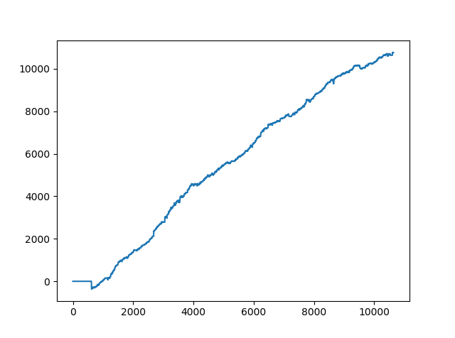
Now this looks good. Our proposed algorithmic trading strategy made 11665 pips. Yes this is 11000 pips in 1 year. At least we didn’t go negative over the span of 10K bars which is equal to almost one year of trading with this algorithmic trading strategy.
>>> #calculate the actual BUY/SELL Impulse Signals
...
>>> for k in range(600,ndf2-2):
...     if (df2['Target(30)'][k-1]==-1.0\
...      and df2['Target(30)'][k]==1.0):
...         df2.ix[k,15]=1.0
...     if (df2['Target(30)'][k-1]==1.0\
...      and df2['Target(30)'][k]==-1.0):
...         df2.ix[k,16]=1.0
...
>>>
>>> #rest Pips to zero
...
>>> df2.Pips=0.0
>>> sum(df2.Pips)
0.0
>>>
>>> sum(df2.Pips)
10759.600000000033
>>>
It appears our Random Forest Algorithmic Trading Strategy is better than the actual. Sounds too good to be true! You can check the Random Forest Algorithmic Trading Strategy code and check. Leave a comment below if you find discrepancies.
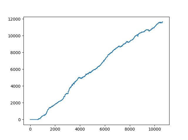
You can see both the equity curves are almost similar. Read this post on how binary options brokers make money. Did you compare the two equity curves? In our RandomForest Algorithmic Trading Strategy, in the start there seems to be a drawdown. We need to check that. Now this RandomForest Algorithmic Trading Strategy is not refined. I will need to work on it more and optimize it more. But you can see in its rough form it still made 11,000 pips in 222 trading days. Overall the algorithmic trading strategy is working well but the drawdown can be as high as 112 pips. In the above algorithmic trading strategy, I didn’t use a stop loss. I will now do the testing with a stop loss.
df2.Pips.astype(bool).sum(axis=0)
df2.Pips[df2.Pips !=0]

def winners(value):
    return max(value, 0)

def drawdown(value):
    return min(value, 0)

df2["winners"] = df2["Pips"].map(winners)
df2["drawdown"] = df2["Pips"].map(drawdown)
sum(df2.winners)
sum(df2.drawdown)
>>> sum(df2.winners)
18253.39999999996
>>> sum(df2.drawdown)
-6587.799999999977
>>> df2.drawdown.min()
-116.20000000000186
plt.plot(df2['drawdown'])
plt.show()
Above I have separate the winners from the losers. As you can see above winners were 18253 pips and drawdown was 6587 pips with the max drawdown 116 pips. We need to use the stop loss and reduce the drawdown. Below is the plot of the drawdown. Drawdown is simply the number of losing trades. Keep this in mind, we are not using a stop loss at this stage.
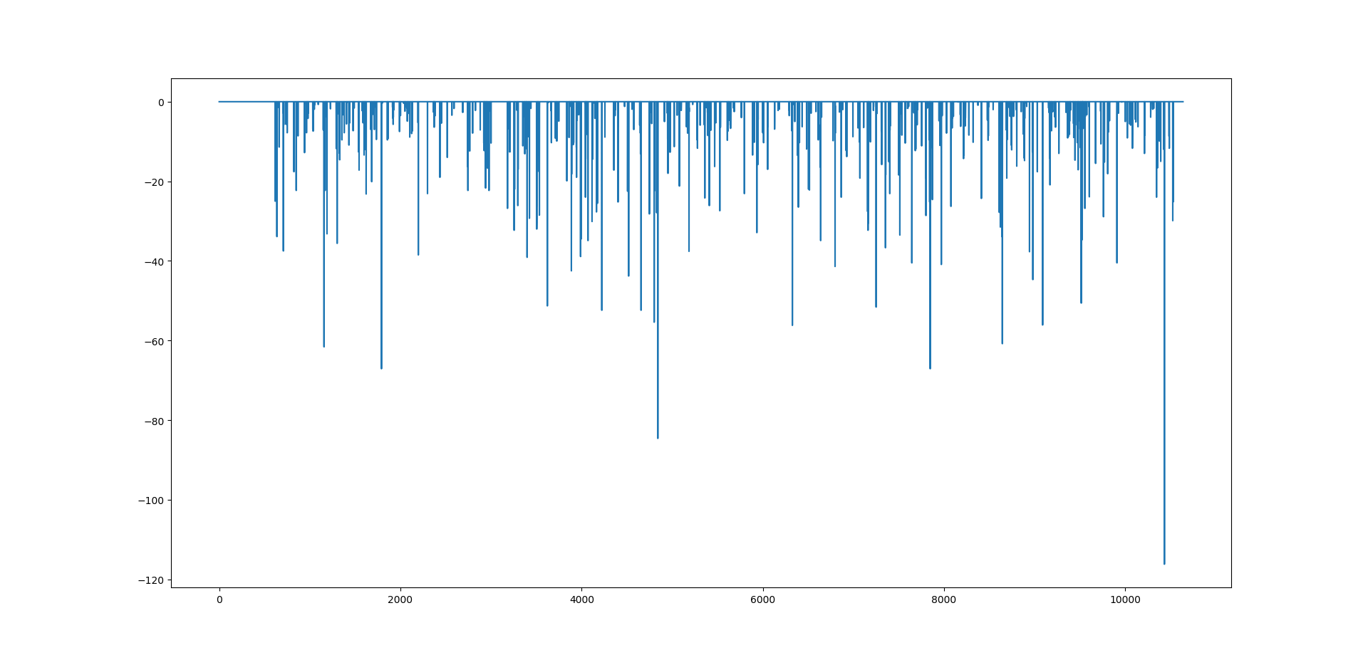
You can see above the line which extends from the rest of the trades. This is the 116 pips drawdown. This is an educational post. The purpose is to show you how to develop algorithmic trading strategies. As you can see with this algorithmic trading strategy we can suffer a max drawdown of 116 pips. Let’s try to reduce the drawdown by using the stop loss. In the first case we place the stop loss at the low for a long trade and at the high for the short trade. Let’s see what happens now!
>>> sum(df2.Pips)
5470.19999999997
>>> def winners(value):
...     return max(value, 0)
...
>>> def drawdown(value):
...     return min(value, 0)
...
>>> df2["winners"] = df2["Pips"].map(winners)
>>> df2["drawdown"] = df2["Pips"].map(drawdown)
>>> sum(df2.winners)
12014.99999999998
>>> sum(df2.drawdown)
-6544.800000000022
>>> plt.plot(df2['drawdown'])
[]
>>> plt.show()
>>> df2.drawdown.min()
-50.89999999999817
>>> df2.winners.max()
259.29999999999785
>>>
As you can see our algorithmic trading strategy has become less profitable with this simple change. The net pips made now have reduced to 5470 pips. But at the same time the max drawdown has also been reduced to 50 pips. This is an illustration of the famous Risk Reward Tradeoff. If you want high return, you will have to take more risk. If you reduce risk the return will also reduce. Let’s change this to close hitting the stop loss and check what happens.
>>> sum(df2.Pips)
7149.699999999986
>>> def winners(value):
...     return max(value, 0)
...
>>> def drawdown(value):
...     return min(value, 0)
...
>>> df2["winners"] = df2["Pips"].map(winners)
>>> df2["drawdown"] = df2["Pips"].map(drawdown)
>>> sum(df2.winners)
12014.99999999998
>>> sum(df2.drawdown)
-4865.299999999991
>>> df2.drawdown.min()
-50.89999999999817
>>> df2.winners.max()
259.29999999999785
Now we have again changed our stop loss strategy. This time the net pips made by the algorithmic trading strategy are 7149 pips and the max drawdown is 50 pips. We have to work more to optimize this algorithmic trading strategy. The core idea of using RandomForest in predicting the price 30 step ahead does seem to work and we can work more on it and see if we can further improve it. This was an educational post. The purpose was to give you an idea how to develop your algorithmic trading strategy. More works needs to done before we can actually use this algorithmic trading strategy in live trading. But as you can see developing algorithmic trading strategies takes your emotions out of the equation. You can measure the performance of your algorithmic trading strategy and can be quite confident how it will perform in live trading. But keep this in mind. All algorithmic trading strategies have an element of surprise in them. The element of surprise in our case is the max drawdown. It was 116 pips. We reduced it to 50 pips. But we need to work more and make sure that our drawdown as lower than 20 pips. I hope you have liked my post on RandomForest Algorithmic Trading Strategy. If you are interested you can check my course Quantitative Trading Fundamentals. In this course, I take you step by step and show you how to develop your algorithmic trading strategies.
>>> #backtesting the trading strategy
... #we start live trading with $100
...
>>> deposit=100
>>> df2['Pips']=0.0
>>> df2.columns.get_loc('Pips')
18
>>> df2['Equity']=0.0
>>> df2.columns.get_loc('Equity')
21
>>> tradeOpen=True
>>> longTrade=False
>>> shortTrade=False
>>> longEntryPrice=0.0
>>> shortEntryPrice=0.0
>>>
>>> stopLoss=0.0
>>> #set the stop loss
...
>>> sl=50
>>>
>>> for k in range(600,ndf2-2):
...     #let's backtest the trading strategy
...     if df2.shortSignal[k]==1.0:
...         if longTrade==True:
...             #close long trade
...             exitPrice=df2.Close.values[k]
...             #open a short trade
...             shortEntryPrice=df2.Close.values[k]
...             stopLoss=df2.Close.values[k]+sl/10000
...             shortTrade=True
...             longTrade=False
...             df2.ix[k,'Pips']=10000*(exitPrice-longEntryPrice)
...     if  df2.longSignal[k]==1:
...         if shortTrade==True:
...             #close short trade
...             exitPrice=df2.Close.values[k]
...             #open a long trade
...             longEntryPrice=df2.Close.values[k]
...             stopLoss=df2.Close.values[k]-sl/10000
...             shortTrade=False
...             longTrade=True
...             df2.ix[k,'Pips']=10000*(shortEntryPrice-exitPrice)
...     if longTrade==False and shortTrade==False:
...         #this is for the first BUY/SELL signal
...         if df2.longSignal[k]==1:
...              #open a long trade
...             longEntryPrice=df2.Close.values[k]
...             stopLoss=df2.Close.values[k]-sl/10000
...             shortTrade=False
...             longTrade=True
...         if df2.shortSignal[k]==1:
...             #open a short trade
...             shortEntryPrice=df2.Close.values[k]
...             stopLoss=df2.Close.values[k]+sl/10000
...             shortTrade=True
...             longTrade=False
...     if longTrade==True:
...         #if df2.Low.values[k] < stopLoss:
...         #if df2.Close.values[k] < stopLoss:
...         if df2.Close.values[k] < stopLoss:
...         #the stop loss has been hit
...         longTrade=False
...         df2.ix[k,'Pips']=10000*(stopLoss-longEntryPrice)
...         stopLoss=0.0
...     if shortTrade==True:
...         #if df2.High.values[k] > stopLoss:
...         #if df2.Close.values[k] > stopLoss:
...         if df2.Close.values[k] > stopLoss:
...             #the stop loss has been hit
...             shortTrade=False
...             df2.ix[k,'Pips']=10000*(shortEntryPrice-stopLoss)
...             stopLoss=0.0
...
>>> sum(df2.Pips)
10764.900000000041
>>> def winners(value):
...     return max(value, 0)
...
>>> def drawdown(value):
...     return min(value, 0)
...
>>> df2["winners"] = df2["Pips"].map(winners)
>>> df2["drawdown"] = df2["Pips"].map(drawdown)
>>> sum(df2.winners)
17946.69999999996
>>> sum(df2.drawdown)
-7181.799999999946
>>> df2.drawdown.min()
-61.59999999999943
>>> df2.winners.max()
259.29999999999785
>>> profitFactor=sum(df2.winners)/abs(sum(df2.drawdown))
>>> profitFactor
2.4989139213010803
>>>
Above I have modified the RandomForest Algorithmic Trading Strategy. I have place a 50 pips stop loss below/above the entry price. Max drawdown has been reduced to 61 pips ( we have halved it from 116 pips). Net pips made is 10764 and the profit factor is 2.5. We need to work more to make our algorithmic trading strategy even more better. Let’s include money management in our testing. We will start with a deposit of $100 and use a universal stop loss of 50 pips for this algorithmic trading strategy. We will be taking 5% risk. Below is the bakctesting code:
>>> #backtesting the trading strategy
... #we start live trading with $100
...
>>> deposit=100
>>> df2['Pips']=0.0
>>> df2.columns.get_loc('Pips')
18
>>> df2['Equity']=0.0
>>> df2.columns.get_loc('Equity')
19
>>> tradeOpen=True
>>> longTrade=False
>>> shortTrade=False
>>> longEntryPrice=0.0
>>> shortEntryPrice=0.0
>>> stopLoss=0.0
>>> equity=deposit
>>> risk=5
>>>
>>> lots=0.0
>>> #set the stop loss
...
>>> sl=50
>>>
>>> for k in range(600,ndf2-2):
...     #let's backtest the trading strategy
...     if df2.shortSignal[k]==1.0:
...         if longTrade==True:
...             #close long trade
...             exitPrice=df2.Close.values[k]
...             #open a short trade
...             shortEntryPrice=df2.Close.values[k]
...             stopLoss=df2.Close.values[k]+sl/10000
...             shortTrade=True
...             longTrade=False
...             lots=(equity*risk/100)/(sl*10)
...             df2.ix[k,'Pips']=10000*(exitPrice-longEntryPrice)
...             equity=equity+df2.Pips[k]*lots*10
...             df2.ix[k,'Equity']=equity
...     if  df2.longSignal[k]==1:
...         if shortTrade==True:
...             #close short trade
...             exitPrice=df2.Close.values[k]
...             #open a long trade
...             longEntryPrice=df2.Close.values[k]
...             stopLoss=df2.Close.values[k]-sl/10000
...             shortTrade=False
...             longTrade=True
...             lots=(equity*risk/100)/(sl*10)
...             df2.ix[k,'Pips']=10000*(shortEntryPrice-exitPrice)
...             equity=equity+df2.Pips[k]*lots*10
...             df2.ix[k,'Equity']=equity
...     if longTrade==False and shortTrade==False:
...         #this is for the first BUY/SELL signal
...         if df2.longSignal[k]==1:
...              #open a long trade
...             longEntryPrice=df2.Close.values[k]
...             stopLoss=df2.Close.values[k]-sl/10000
...             df2.ix[k,'Equity']=deposit
...             shortTrade=False
...             longTrade=True
...         if df2.shortSignal[k]==1:
...             #open a short trade
...             shortEntryPrice=df2.Close.values[k]
...             stopLoss=df2.Close.values[k]+sl/10000
...             df2.ix[k,'Equity']=deposit
...             shortTrade=True
...             longTrade=False
...     if longTrade==True:
...         #if df2.Low.values[k] < stopLoss:
...         #if df2.Close.values[k] < stopLoss:
...         if df2.Close.values[k] < stopLoss:
...    #the stop loss has been hit
...    longTrade=False ... lots=(equity*risk/100)/(sl*10)
...    df2.ix[k,'Pips']=10000*(stopLoss-longEntryPrice)
...    equity=equity+df2.Pips[k]*lots*10
...    df2.ix[k,'Equity']=equity
...    stopLoss=0.0
...    if shortTrade==True:
...    #if df2.High.values[k] > stopLoss:
...         #if df2.Close.values[k] > stopLoss:
...         if df2.Close.values[k] > stopLoss:
...             #the stop loss has been hit
...             shortTrade=False
...             lots=(equity*risk/100)/(sl*10)
...             df2.ix[k,'Pips']=10000*(shortEntryPrice-stopLoss)
...             equity=equity+df2.Pips[k]*lots*10
...             df2.ix[k,'Equity']=equity
...             stopLoss=0.0
...
>>> equity
3042429.984101838
Wow! Our RandomForest Algorithmic Trading strategy made $3 Million starting with a deposit of $100. Sounds too good to be true! Maybe!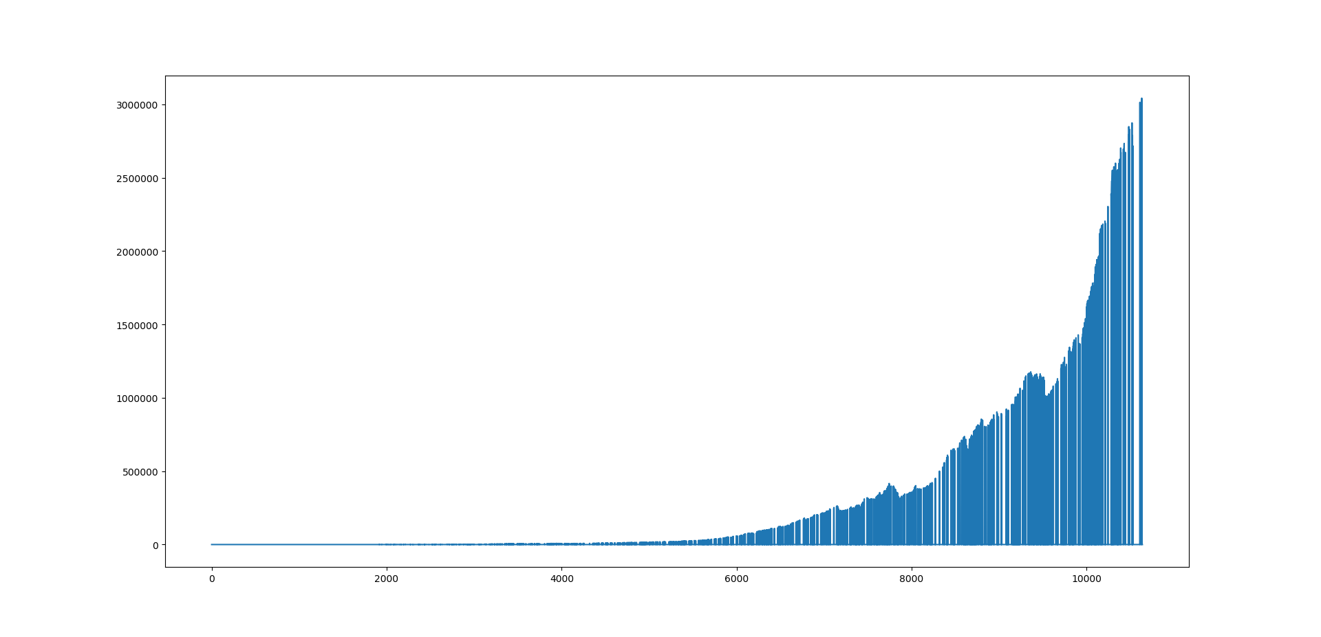 Above is the equity curve. How did we manage to convert $100 into $3M in just 1 year? It was the power of compounding that made this possible. Our risk is always 5%. We keep on increasing the lot size as our account equity increases. This is a good illustration of how compounding can help you make a fortune. Good Luck! But everything sounds to good to be true. I rechecked the RandomForest Algorithmic Trading Strategy. I had made one mistake that was giving these fantastic results. I made the correction and viola the number of pips made by this algorithmic trading strategy dropped to just 534. Read the post and figure out what mistake I had made and how it was giving fantastic results. I hope you enjoyed reading my post.
UPDATE: Now you might be wondering wow we got fantastic results what was the wrong thing that we did that gave us these wonderful results. This algorithmic trading model is suffering from LOOK AHEAD BIAS also known as PEEKING BIAS. We have been looking into the future when making the predictions. It is just like predicting the intraday prices knowing the daily closing price when actually you don’t know it till the end of the day. So what we were doing we were taking the future data into account when trying to predict the future. This is something that often happens when you don’t check you algorithmic trading model carefully. When you when get a very nice equity curve that we did like above, it is time to double check your algorithmic trading model. We got such a fantastic equity curve because we were predicting the future while already knowing what it would be. These types of mistakes are easy to spot when you get fantastic results. Other types of errors that you can make while backtesting algorithmic trading models are the DATA MINING BIAS and the OVER OPTIMIZATION BIAS. Over optimization bias is also known as the CURVE FITTING BIAS. This happens when you try to overfit the model to the trading data and it overfits on the randomness in the training data. Always keep this in mind that overfitting is a major issue in the world of machine learning. Most of the time you will be trying to avoid it by using L1 and L2 regularization.